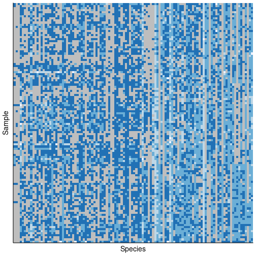
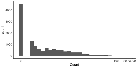
class: center, middle, inverse, title-slide # Transformations for count data ### Mahendra Mariadassou, INRAE ### Shandong University, Weihai (CN)<br>Summer School 2021 --- <script type="text/x-mathjax-config"> MathJax.Hub.Config({ TeX: { Macros: { P: "{\\mathcal{P}}", N: "{\\mathcal{N}}", M: "{\\mathcal{M}}", D: "{\\mathcal{D}}", LN: "{\\mathcal{LN}}", Rbb: "{\\mathbb{R}}", Nbb: "{\\mathbb{N}}", Sbb: "{\\mathbb{S}}", bpi: "{\\boldsymbol{\\pi}}", bp: "{\\mathbf{p}}", bg: "{\\mathbf{g}}", bm: "{\\mathbf{m}}", bn: "{\\mathbf{n}}", bo: "{\\mathbf{o}}", bs: "{\\mathbf{s}}", bx: "{\\mathbf{x}}", bA: "{\\mathbf{A}}", bB: "{\\mathbf{B}}", bM: "{\\mathbf{M}}", bS: "{\\mathbf{S}}", bX: "{\\mathbf{X}}", bY: "{\\mathbf{Y}}", bZ: "{\\mathbf{Z}}", balpha: "{\\boldsymbol{\\alpha}}", bbeta: "{\\boldsymbol{\\beta}}", bfeta: "{\\boldsymbol{\\eta}}", bgamma: "{\\boldsymbol{\\gamma}}", bphi: "{\\boldsymbol{\\phi}}", btau: "{\\boldsymbol{\\tau}}", btheta: "{\\boldsymbol{\\theta}}", bTheta: "{\\boldsymbol{\\Theta}}", bmu: "{\\boldsymbol{\\mu}}", bSigma: "{\\boldsymbol{\\Sigma}}", bOmega: "{\\boldsymbol{\\Omega}}" } } }); </script> --- class: middle # Reminder .pull-left[ - Interest for .alert[multivariate count data] - Counts in ecology have .alert[peculiar] features: - sparse (.grey[grey cell] = null count) - overdispersed - not centered around a central location parameter - Example from Jakuschkin, Fievet, Schwaller, Fort, Robin, and Vacher [Jak+16] <img src="02_transformation_files/figure-html/oaks_histo-1.png" width="800px" /> ] .pull-right[ <!-- --> ] --- class: inverse, middle, center # Transformations --- # Data transformations - Many classic transformations to turn .alert[counts] into continuous .alert[pseudo-gaussian] values: - `\(\arcsin(\sqrt{x})\)` - `\(\log(x)\)` - `\(\sqrt{x}\)` - `\(\text{xlr}(x)\)` where x is either **c** for centered or **i** for isometric log-ratio - etc -- Each transformation has its own .alert[rationale] but they are all based on the .alert[Poisson] or .alert[binomial / multinomial] distribution and are more or less efficient. -- <!-- --> --- # About the Poisson distribution A Poisson random variable `\(X\)` with parameter `\(\lambda = e^\theta\)`, noted `\(X \sim \mathcal{P}(\lambda)\)` is defined by: - `\(X \in \mathbb{N}\)` - `\(\forall n \in \mathbb{N}, P(X = n) = e^{-\lambda}\frac{\lambda^n}{n!} = \exp(n\theta - e^\theta - \log(n!))\)` -- In particular, - `\(E[X] = \lambda\)` - `\(V[X] = \lambda\)` - `\(E[e^{tX}] = e^{\lambda(e^t - 1)}\)` (moment generating function) The Poisson distribution is **closed under independent sums**: if `\(X_1\)` and `\(X_2\)` are independent Poisson with `\(X_1 \sim \mathcal{P}(\lambda_1)\)` and `\(X_2 \sim \mathcal{P}(\lambda_2)\)`, then `\(X_1 + X_2 \sim \mathcal{P}(\lambda_1 + \lambda_2)\)` -- The variance increases with the mean: search for .alert[variance stabilizing] transformations `\(\rightarrow\)` `\(Y = f(X)\)` such that `\(V[Y]\)` is constant. --- ### Closure: direct computation <img src="ext_figures/poisson_closure_direct.png" width="100%" /> --- ### Closure: moment generating function <img src="ext_figures/poisson_closure_mgf.png" width="100%" /> --- # Square root: delta method - If `\(g\)` is a function with continuous first derivative such that `\(g'(\mu) \neq 0\)` - If `\(X_1, \dots, X_n\)` are independent copies of a r.v. `\(X\)` with mean `\(\mu\)` and variance `\(v\)` - If we note `\(\bar{X}_n = \frac{X_1 + \dots + X_n}{n}\)` Then $$ \sqrt{n}\left( g(\bar{X}_n) - g(\mu)\right) \xrightarrow[n \to \infty]{d} \mathcal{N}\left(0, v g'(\mu)^2\right) $$ -- Demo based on Taylor expansion .alert[see next slide] --- <img src="ext_figures/delta_method.png" width="100%" /> --- ### Application to Poisson variables In the case of Poisson r.v. the equality becomes $$ \sqrt{n}\left( g(\bar{X}_n) - g(\lambda)\right) \xrightarrow[n \to \infty]{d} \mathcal{N}\left(0, \lambda g'(\lambda)^2\right) $$ Therefore, if we set `\(g'(\lambda) = \lambda^{-1/2}\)`, and thus `\(g(\lambda) = 2\sqrt{\lambda}\)` $$ 2 \sqrt{n \bar{X}_n} - 2\sqrt{n\lambda} \xrightarrow[n \to \infty]{d} \mathcal{N}(0, 1) $$ By closedness, if the `\(X_i\)` are i.i.d with distribution `\(\mathcal{P}(\lambda/n)\)`, then `\(n\bar{X}_n \sim \mathcal{P}(\lambda)\)` and the second term on the left-hand side is equal to `\(2\sqrt{\lambda}\)`, which justifies the approximation $$ 2\sqrt{X} \simeq \mathcal{N}\left(2\sqrt{\lambda}, 1\right) $$ -- For better results for low values of `\(\lambda\)`, the [Anscombe transform](http://www.jstor.org/stable/2984159) uses `\(\tilde{g}(\lambda) = 2\sqrt{\lambda + \frac{3}{8}}\)` --- # Jensen inequality If `\(f\)` is strictly concave on `\(I \subset \Rbb\)` and `\(X\)` is a `\(I\)`-valued random-variable: $$ E[f(X)] \leq f(E[X]) $$ with equality if and only if `\(X = E[X]\)` almost surely. --- # Log transformation The rationale for log transformation is less clear and mostly stems from it belonging to the family exponential distributions. If we note `\(\theta = \log(\lambda) \Leftrightarrow e^\theta = \lambda\)` $$ P(X = n) = e^{-\lambda}\frac{\lambda^n}{n!} = \exp(n\theta - e^\theta - \log(n!)) $$ And thus `\(\theta = \log(\lambda)\)` is the .alert[natural parameter] of the Poisson distribution, `\(X\)` the .alert[sufficient statistic] and `\(\log\)` the natural .alert[link function]. -- Since `\(E_{\theta}[X] = e^\theta \Rightarrow \log(E_\theta(X)) = \theta\)`, it can be natural to think that `\(E[\log(X)] \simeq \theta\)`. The `\(\log\)` transform is also widely used in many fields so it can feel natural to work on log-counts. --- # Log transformation (II) But Jensen's inequality for concave functions implies $$ E[\log(X)] < \log \left( E[X] \right) $$ so the transformation is biased. It is also problematic for .alert[sparse data] as `\(\log(0)\)` is not defined. -- The usual workaround is to consider `\(\log(X + c)\)` for a small `\(c\)` but it also systematic bias in the data (a huge mass in `\(\log(c)\)`) as illustrated below for `\(\log(x+1)\)`. .center[ <!-- --> ] --- # Arcsin (square-root) transform The `\(\arcsin(\sqrt{x})\)` transform assumes that data are .alert[compositional] and reflect .alert[proportions]. It is _approximately_ **variance stabilizing** for **binomial proportions**. -- Assume that `\(X \sim \mathcal{B}(n, p)\)` and is a sum of `\(n\)` i.i.d Bernoulli r.v. `\(\mathcal{B}(p)\)`. Note `\(\hat{p} = X/n\)`. Using the CLT and the delta method, we have for every continuous function `\(g\)` with non zero derivative at `\(p\)`. $$ \sqrt{n}\left(g(\hat{p}) - g(p)\right) \xrightarrow[n \to \infty]{d} \mathcal{N}\left(0, p(1-p) g'(p)^2\right) $$ We can make the variance constant by taking `\(g'(p) = \frac{1}{\sqrt{p(1-p)}}\)` which is the derivative of `\(g(p) = 2\arcsin(\sqrt{p})\)`. -- `\(2\arcsin(\sqrt{\hat{p}})\)` is thus approximately gaussian $$ 2\arcsin(\sqrt{\hat{p}}) \simeq \N\left(2\arcsin{\sqrt{p}}, \frac{1}{n}\right) $$ But the approximation is worst for values of `\(p\)` close to `\(0\)` and `\(1\)` [WH11]. --- # Centered log-ratio Assumes that data are .alert[compositional] and reflect .alert[proportions]. -- The **centered log-ratio** maps the **probability simplex** `\(\Sbb^{p-1} = \{ (s_1, \dots, s_p) \in (0,1)^p \text{ s.t. } \sum_i s_i = 1\}\)` (or space of compositions) to a linear subspace `\(E\)` of `\(\Rbb^p\)` of dimension `\(p-1\)`, orthogonal to `\((1, \dots, 1)\)` and defined by `\(\{ (x_1, \dots, x_p) \in \Rbb^p \text{ s.t. } \sum_i x_i = 0\}\)`. $$ clr: `\begin{align} \quad & \Sbb^{p-1} & \to & E \subset \Rbb^p \\ & \mathbf{s} & \mapsto & clr(\mathbf{s}) = \left( \log\left(\frac{s_1}{G(\mathbf{s})}\right), \dots, \log\left(\frac{s_1}{G(\mathbf{s})}\right) \right) \text{with} \; \log(G(\mathbf{s})) = \frac{1}{n} \sum_i \log(s_i) \end{align}` $$ <img src="ext_figures/clr_transform.png" width="85%" style="display: block; margin: auto;" /> --- ## Rationale - First introduced by Aitchison [Ait86] - Since the probabilities sum up to 1, their absolute values are not informative but their (log)-ratio are. - The compositions can in facts sum up to any (positive) values, the clr transform is **scale-invariant** - However clr transform is .alert[not subcompositional]: it changes when considering only part of the data. --- # Scale invariance of clr <img src="ext_figures/scale_invariance.png" width="100%" style="display: block; margin: auto;" /> --- # Centered log-ratio **Problems with ecology data** - Compositions are not observed directly but only through .alert[noisy counts]. - A composition `\(\hat{s}\)` estimated from count data can be quite far from the actual composition `\(\mathbf{s}\)`. - Computing log-ratio from null counts is not feasible - Adding a small .alert[pseudo-count] to all counts before computing proportions does .alert[not preserve] scale invariance -- .pull-left[ - Proportions `\(s = (0.1, 0.4, 0.5)\)` - Observed counts `\(n = (2, 3, 5)\)` - Observed proportions `\(\hat{p} = (0.2, 0.3, 0.5)\)` - With pseudocounts `\(\tilde{p} = (0.23, 0.31, 0.46)\)` ] .pull-right[ - `\(clr(p) = (-0.999, 0.388, 0.611)\)` - `\(clr(n) = (-0.441, -0.035 , 0.476)\)` - `\(clr(\hat{p}) = clr(n)\)` and `\(clr(\tilde{p}) = clr(n+1)\)` - `\(clr(\tilde{p}) = (-0.327, -0.039, 0.366)\)` ] --- # Remarks - The tranformations are mostly .alert[univariate], except clr - All transformations work well - for Poisson distributions with large `\(\lambda\)` - for binomial distributions with proportion `\(p\)` close to `\(1/2\)` - They fail for .alert[small counts], which are frequent in ecology - Compositions - Log-transformation (centered or not) requires .alert[special handling] of 0s -- The results is not always perfect <!-- --> --- # Better alternatives - The transformations are applied .alert[directly to the data] - it's fast with some statistical grounding - used to improve .alert[linearity of the response] and .alert[homogeneity of the variance] (homoscedasticity). - kind of .alert[preprocessing] before using standard multivariate techniques for gaussian data -- - In many cases (log transform for Poisson variables), it makes more sense to apply it to the .alert[expected value] or the .alert[parameter]. $$ `\begin{equation} X \sim \P(e^\theta) \Rightarrow \log(E[X]) = \theta \; \text{ but not } \; E_{\theta}[\log(X)] = \theta \end{equation}` $$ - That's the rationale behind .alert[generalized linear models] -- - O’Hara and Kotze [OK10] compared - linear normal (LM) on transformed data - generalized linear models (GLM) on original data - and found that GLM outperformed LM (except for large counts and small oversdispersion). --- class: center, middle <div class="figure"> <img src="ext_figures/mee3_21_f3.gif" alt="Estimated root mean-squared error from six different models, applied to data simulated from a negative binomial distribution. Decreasing r indicates greater variances. Taken from [OK10]" width="70%" /> <p class="caption">Estimated root mean-squared error from six different models, applied to data simulated from a negative binomial distribution. Decreasing r indicates greater variances. Taken from [OK10]</p> </div> --- Aitchison, J. (1986). _The Statistical Analysis of Compositional Data_. Springer Netherlands. DOI: [10.1007/978-94-009-4109-0](https://doi.org/10.1007%2F978-94-009-4109-0). URL: [https://doi.org/10.1007/978-94-009-4109-0](https://doi.org/10.1007/978-94-009-4109-0). Jakuschkin, B., V. Fievet, L. Schwaller, et al. (2016). "Deciphering the pathobiome: intra-and interkingdom interactions involving the pathogen Erysiphe alphitoides". In: _Microbial ecology_ 72.4, pp. 870-880. O’Hara, R. B. and D. J. Kotze (2010). "Do not log-transform count data". In: _Methods in Ecology and Evolution_ 1.2, pp. 118-122. URL: [https://doi.org/10.1111/j.2041-210X.2010.00021.x](https://doi.org/10.1111/j.2041-210X.2010.00021.x). Warton, D. I. and F. K. C. Hui (2011). "The arcsine is asinine: the analysis of proportions in ecology". In: _Ecology_ 92.1, pp. 3-10. URL: [https://doi.org/10.1890/10-0340.1](https://doi.org/10.1890/10-0340.1).