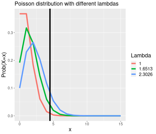
class: center, middle, inverse, title-slide .title[ # Tests ] .author[ ### Mahendra Mariadassou, INRAE <br> .small[from original slides by Tristan Mary-Huard] ] .date[ ### Shandong University, Weihai (CN)<br>Summer School 2023 ] --- <script type="text/x-mathjax-config"> MathJax.Hub.Config({ TeX: { Macros: { P: "{\\mathcal{P}}", B: "{\\mathcal{B}}", L: "{\\mathcal{L}}", F: "{\\mathcal{F}}", N: "{\\mathcal{N}}", M: "{\\mathcal{M}}", D: "{\\mathcal{D}}", LN: "{\\mathcal{LN}}", Rbb: "{\\mathbb{R}}", Nbb: "{\\mathbb{N}}", Sbb: "{\\mathbb{S}}", bpi: "{\\boldsymbol{\\pi}}", bp: "{\\mathbf{p}}", bg: "{\\mathbf{g}}", bm: "{\\mathbf{m}}", bn: "{\\mathbf{n}}", bo: "{\\mathbf{o}}", bs: "{\\mathbf{s}}", bx: "{\\mathbf{x}}", bA: "{\\mathbf{A}}", bB: "{\\mathbf{B}}", bM: "{\\mathbf{M}}", bS: "{\\mathbf{S}}", bX: "{\\mathbf{X}}", bY: "{\\mathbf{Y}}", bZ: "{\\mathbf{Z}}", balpha: "{\\boldsymbol{\\alpha}}", bbeta: "{\\boldsymbol{\\beta}}", bfeta: "{\\boldsymbol{\\eta}}", bgamma: "{\\boldsymbol{\\gamma}}", bphi: "{\\boldsymbol{\\phi}}", btau: "{\\boldsymbol{\\tau}}", btheta: "{\\boldsymbol{\\theta}}", bTheta: "{\\boldsymbol{\\Theta}}", bmu: "{\\boldsymbol{\\mu}}", bSigma: "{\\boldsymbol{\\Sigma}}", bOmega: "{\\boldsymbol{\\Omega}}" } } }); </script> --- class: middle, inverse, center # Warm-up ## Introducing the Fisher distribution --- ## Prerequesites: Fisher distribution Let `\(Z_1\)` and `\(Z_2\)` be two positive random variables such that - `\(Z_1\sim\chi^2(n_1)\)`, - `\(Z_2\sim\chi^2(n_2)\)`, - `\(Z_1\perp Z_2\)`. Define `$$F = \frac{Z_1/n_1}{Z_2/n_2}$$` -- Then `\(F\)` is said to follow a Fisher distribution with degrees of freedom `\(n_1\)` and `\(n_2\)`. One notes `$$F \sim \F(n_1,n_2)$$` --- ## Example 1: Infection Back to the phage infection example. Assume now that if at least 90% of the bacteria colony is infected then the biologist applies a treatment to fight the infection. What decision rule should be applied ? ``` 2 2 2 2 3 3 2 4 1 1 5 1 3 1 1 5 1 1 4 2 ``` .blue[Objective] Perform a test to decide whether the proportion of infected bacteria is higher than `\(90\%\)` or not. --- ## Modeling Denote `\(X_i\)` the number of phages obtained for the `\(i^{th}\)` bacterium. - One assumes that bacteria are independent: `\(X_1 \perp X_2 \perp \dots \perp X_{n},\quad\text{with } n= 20\)` - Measurements are discrete `\(X_1,..., X_{n} \sim \mathcal{P}(\bullet), \text{ i.i.d}\)` - The infection level is unknown `\(X_1,..., X_{n} \sim \mathcal{P}(\lambda), \text{ i.i.d}\)` --- ## Hypotheses Hypotheses *must* be formulated such that they *concern a parameter* of the model. Here the model is `$$X_1,..., X_{n} \sim \mathcal{P}(\lambda), \text{ i.i.d}$$` Consequently the hypotheses should concern `\(\lambda\)`. -- `$$\begin{eqnarray*} \hspace{-0.8cm}\text{Proportion of infected bacteria } \geq \text{90\%} &\Rightarrow& P(X>0)\geq 0.9 \\ &\Rightarrow& P(X=0)\leq 0.1 \\ &\Rightarrow& e^{-\lambda}\leq 0.1 \\ &\Rightarrow& \lambda\geq -\ln(0.1) \\ &\Rightarrow& \lambda\geq \lambda_0 (=2.3026) \\ \end{eqnarray*}$$` -- Hence `$$H_0: \{\lambda\leq \lambda_0\} \quad \text{vs} \quad H_1: \{\lambda\geq \lambda_0\}$$` --- ## Estimation Starting point: derive the ML estimator for the quantity of interest. `$$\begin{eqnarray*} Lik_\lambda(x_1,...,x_n) &=& \prod_{i=1}^n f_\lambda(x_i) \quad\text{(i.i.d. assumption)}\\ &=& \prod_{i=1}^n \frac{\lambda^{x_i}}{x_i!}e^{-\lambda} \\ \Rightarrow LLik_\lambda(x_1,...,x_n) &=& \log(\lambda)\sum_{i=1}^{n}x_i - \sum_{i=1}^{n}\log(x_i!) - n\lambda \end{eqnarray*}$$` .blue[Derivation] `$$\frac{\partial LLik_\lambda(x_1,...,x_n)}{\partial \lambda}= \frac{1}{\lambda}\sum_{i=1}^n x_i -n$$` Setting the derivative at 0, one gets: `\(\widehat{\lambda} = \frac{1}{n}\sum_{i=1}^n x_i=\bar{x}\)`. --- ## Decision rule Should be of the form `$$\text{If } \hat{\lambda}\geq s \text{ then reject } H_0$$` One needs to choose threshold `\(s\)`. .blue[Type I error control] Find `\(s\)` such that `\(P_{H_0}(\overline{X}\geq s)\leq \alpha\)` `\(\Rightarrow\)` Requires the (possibly approximate) distribution of `\(\overline{X}\)`. One has: `$$\begin{eqnarray*} n\overline{X} \sim \P(n\lambda) \quad \text{ and/or } \quad \sqrt{n}\frac{\overline{X}-\lambda}{\lambda} \overset{approx}{\sim} \N(0,1) \end{eqnarray*}$$` .blue[Under `\(H_0\)`]: One has `\(\lambda \in [0,\lambda_0]\)`, still the `\(H_0\)` distribution of `\(\overline{X}\)` is not fully known... --- ## Worst case scenario Which value of `\(\lambda \in [0,\lambda_0]\)` leads to the worst (i.e. the max) value of `\(P_{H_0}(\overline{X}\geq s)\)` ? <!-- --> -- Worst value: `\(\lambda =\lambda_0\)` ! --- ## Back to the decision rule Considering the worst case scenario, one looks for `\(s\)` such that `$$P_{\lambda_0}\left( \overline{X}\geq s \right)\leq \alpha \Rightarrow P_{\lambda_0} \left( n\overline{X}\geq ns \right)\leq \alpha$$` Choose `\(ns = q_{n\lambda_0,1-\alpha} \Rightarrow s = \frac{q_{n\lambda_0,1-\alpha}}{n}\)`, .blue[Application] - `\(\widehat{\lambda}=\)` 2.3 - `\(n=\)` 20 - `\(\alpha= 0.05\)` - `\(q_{n\lambda_0,1-\alpha}=\)` 57 `\(\Rightarrow s=\)` 2.85 -- .blue[Conclusion ?] One does not reject the hypothesis that the proportion of infected bacteria is lower than 90\% --- ## Power of a test procedure Recall that the test procedure is design such that: - T1E is controlled at a given level, - T2E is minimum given T1E is controlled. T2E is minimum `\(\Rightarrow\)` `\(P_{H_1}( \text{accept } H_0)\)` is minimum `\(\Rightarrow\)` `\(P_{H_1}(\text{reject} H_0)\)` is maximum. `\(P_{H_1}(\text{reject } H_0)\)` is the ability to reject `\(H_0\)` when it false. This key quantity is called the __power__ of the test procedure.